Simple sequential refinement

The purpose of this tutorial is to familiarize you with the basic functions of the Viewer.

Import

P61A beamline saves spectra as NeXuS .nxs files and metadata as FIO .fio files. The beamline conrtrol software SPOCK is set up in such a way, that if you make a single acquisition using ct command, just one .nxs file will be saved, and if you make a scan (ascan, dscan, mesh, etc.), a .fio file with motor positions will be created, and next to it a directory by the same name with the .nxs files collected at different motor positions.

In P61A::Viewer you can import just NeXuS files (without motor positions and other metadata) and FIO files (with all corresponding spectra and metadata) using the + button.

For this tutorial we have prepared a simple dataset you can download here. As a first step, import the dataset by pressing the + button on the Viewer and selecting the FIO file.

Project files

After you have imported the data, you should save your analysis using File -> Save As menu. The format of the project files is .pickle, and they are just serialized Python 3 objects.

Project files are cross-platform and self-sufficient: you do not need to store them next to the collected data and can transfer them from one computer to another.

Warning

P61A Toolkit is a young project with high expectancy of bugs! Software may freeze or crash. To avoid frustration, please save your analysis regularly.

View / Sort

The dataset for this tutorial is called sdp_00001, which stands for Shifting Double Peaks. Purpose of this tutorial is to show you how P61A::Viewer treats peaks during sequential refinement.

First step of sequential refinement is organizing your data. You can sort the datasets by name, detector dead time, fit quality, and metadata values by clicking on the column headers of the dataset table. You can also add / remove columns from the table by right-clicking the header, and selecting metadata variables in the popup menu.

In this dataset values for eu.x, eu.y and eu.z are random. You can sort the data by them to see how it looks, but to continue we need to have data sorted by Name or xspress3_index.

Peak search

The peak search algorithm in P61A::Viewer searches for local maxima in the datasets, and then filters them by the following criteria:

1. Height: Minimal height of the point to be considered a peak.

2. Distance: Minimal distance between two peaks in keV.

3. Width: Minimal width (FWHM) of the peak in keV.

4. Prominence: Minimal distance between the peak and the surrounding baseline.

If you want to learn more about the algorithm, you can find its description here.

For the tutorial dataset the appropriate parameters are: Height 1000., Distance 2., Width 0.3, Prominence 800.. After you have set the values, press Find button and perform the search over all spectra.

To get a sense of what these parameters mean, we recommend you play around with the values: change them one by one, repeat the search, and see at what value of each parameter peaks start disappearing.

Peak tracking

After the peak search has found all appropriate peaks in all specified spectra, you can organize peaks into tracks. Tracks should follow the same physical peak over all analysed spectra. Since different datasets may have different variance in peak positions between spectra, you have to define the Track window: maximal distance between the peak positions in the neighbouring spectra. The algorithm connects two closest peaks in the neighbouring spectra if the distance between them is less than the Track window value.

For the tutorial dataset to be tracked properly, the Track window should be set to 1. When you press Make tracks button, tracks should appear on the plot. To understand what exactly Track window does, try playing around with it, increase or decrease it.

Peak refinement

To refine the automatically generated peak positions, go to the Peak fit tab.

Every peak has a set of refineable parameters, and a set of non-refineable parameters. At the moment only pseudo-Voigt peak shape approximation is available in the Viewer, with the refineable parameters: center, amplitude, sigma, fraction. Non-refineable parameters are: width, height, base, overlap base, Rwp, chi2.

The peak function follows the definition:

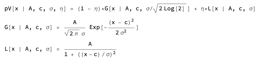
Width is calculated as FWHM, height is the max value of the peak function.

Base defines the peak function domain and is measured in sigmas. Every peak function is calculated according to the pseudo-Voigt expression within its domain [center - base * sigma, center + base * sigma] and is set as 0 outside the domain. The way refinement works in P61A::Viewer is that every peak is only evaluated and refined over its base. Usually base values between 3 and 7 give good results, depending on the peak’s “skirt” and surrounding background. The choice of base value depends on each dataset and each peak.

Parameter overlap_base is also measured in sigmas and determines if peaks next to each other should be refined together or separately: if for two peaks their overlap bases do in fact overlap, they will be refined together on an interval made from combining their bases. By default overlap_base is set relatively small, so that every peak is refined on its own. However, if you notice a drop in fit quality due to a couple of peaks being interdependent, increasing their overlap_base until they are refined together may solve the issue.

In addition to the refineable parameters, base, and overlap_base there are also convenience parameters like height and width, and per-peak fit quality metrics rwp2 and chi2.

The dataset for this tutorial is relatively uncomplicated, so the automated peak search has done a good job initiating the peak parameters. The only thing left to do is to launch the refinement:

• Fit peaks will refine peak parameters in the current spectra,

• Fit Background will do nothing in this dataset, since we have not added any background models

• Fit this will run peak and background fits in sequence until convergence is reached

• Fit multiple will let you run any of the options above on multiple spectra with additional options like initiating all fit models from current one.

For this dataset if you just run Fit multiple in its default mode on all spectra you should get reasonable fit quality.

Peak export

After you are happy with the quality of the refinement, you can export the results using Export peaks button. It is not important for the purposes of this tutorial, but will be important further on.