Plots

Pydidas uses ESRF’s silx toolkit for plotting, with some minor additional functionality. The individual plots are presented below:

Pydidas 2D plot

The PydidasPlot2d is a subclassed silx Plot2d with additional features useful in pydidas.

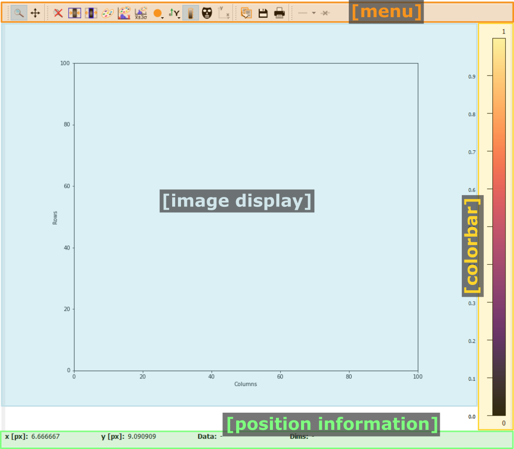
• The menu

  The menu bar allows access to all generic silx and additional pydidas functionality. The detailed menu icons and actions are described below in the menu entries description.

• The image display

  This widget shows the image data. Depending on the zoom level, this is either the full image or a sub-region.

• The colorbar

  The colorbar shows the reference for the used colormap to map data levels to colors.

• The position information

  This widget displays the coordinates and data values of the data under the mouse cursor.

Two-dimensional plots are presented in a silx Plot2D widget. The toolbar options will be explained in detail below. Moving the mouse over the canvas will update the labels for x/y position and data value at the bottom of the canvas. Note that the x and y axis positions for each pixel are defined at the pixel center and the given values must be treated carefully with respect to the pixel shape, especially for coarse pixels.

Tip

Scaling of the results can be achieved by modifying the colormap settings.

Menu entries description

Menu icon	Description
	Zoom mode: clicking with the mouse and dragging spans a new selection of the data to be visualized.
	Panning mode: clicking with the mouse and dragging moves the data on the canvas.
	Unzoom: Reset the display region to the full data.
or	Lock the zoom at the current settings. The button will show the current lock state in its icon and description and a click will toggle between the locked and unlocked state. When the zoom is locked, the display region will not change when loading new data.
or	Toggle the canvas size. Clicking this button will toggle between the two options and change the icon accordingly. Options are a. Match canvas and b. Expand canvas. Match canvas to the data: Set the aspect ratio to 1 and match the canvas size to the data to allow a tight fit. Or Expand the canvas: Reset the canvas size to take up all available space. This option does also change the data aspect ratio to make use of the full canvas.
	Open the colormap editor: This button opens a window with selections for the colormap and scaling of the displayed minimum and maximum values.
	Crop histogram outliers: Calculate the histogram of the image and set the colormap to ignore the low x% and the top y% of the image histogram. The levels of x and y can be adjusted in the pydidas user settings.
	Autoscale the colormap to the image minimum and maximum values.
	Autoscale the colormap to the image mean value +/- 3 standard deviations.
	This action allows to control the aspect of the displayed data and allows to stretch the data to fill the available canvas or keep its original aspect ratio.
	Control the position of the origin in the image: Select between the top left and bottom left corner.
	Display or hide the colorbar on the drawing canvas.
	Mask tools: This button opens an additional widget at the bottom of the canvas with tools for importing or setting a mask to mask certain data regions.
	Set coordinate system: This button will open a submenu which allows to select the coordinate system (cartesian or cylindrical). Note that the cylindrical coordinate system uses the global DiffractionExperimentContext calibration to determine the beam center. Therefore, looking at data with a different calibration will display a wrong center and consequently wrong coordinates.
	Get information for selected datapoint: This button allows the user to click on a point in the image and show a window with additional information about this point (specifically: all indices / data values).
	Copy the currently visible figure to the clipboard. This will only copy the main figure and not the colorbar.
	Save the currently loaded full data to file, ignoring any zooming. This function will open a dialogue to select the file type and filename. Depending on the selected file type, the colormap and scaling will be retained (e.g. for png export) or ignored (e.g. tiff export).
	Print the currently visible figure. This will print only the data visible on the canvas and it will retain colormap and scaling settings.
	Create and delete line profiles. This function allows the selection and editing of line profiles. The line profiles are shown in the histogram plots for the vertical and horizontal axes, respectively.

Pydidas 1D plot

The PydidasPlot1d is a subclassed silx Plot1d with additional features useful in pydidas.

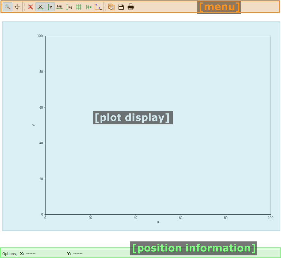
• The menu

  The menu bar allows access to all generic silx and additional pydidas functionality. The detailed menu icons and actions are described below in the menu entries description.

• The plot display

  This plot shows the data. Depending on the zoom level, this is either the full image or a sub-region.

• The position information

  This widget displays the coordinates and data values of the data under the mouse cursor.

Menu entries description

Menu icon	Description
	Zoom mode: clicking with the mouse and dragging spans a new selection of the data to be visualized.
	Panning mode: clicking with the mouse and dragging moves the data on the canvas.
	Unzoom: Reset the display region to the full data.
or	Lock the zoom at the current settings. The button will show the current lock state in its icon and description and a click will toggle between the locked and unlocked state. When the zoom is locked, the display region will not change when loading new data.
	Activate autoscaling of the x-axis: If enabled, the x-axis will be matched to the data range upon activation or upon using the “Unzoom” button.
	Activate autoscaling of the y-axis: If enabled, the y-axis will be matched to the data range upon activation or upon using the “Unzoom” button.
	Switch between a linear and a logarithmic x-axis.
	Switch between a linear and a logarithmic y-axis.
	Toggle a grid in the main plotting canvas.
	Change the drawing style. Repeatedly using this button will cycle through lines, dots, and lines & dots styles for the curve.
or	Change the plot style: Switch between a standard y vs. x or a Kratky-type plot. The Kratky-type plot uses y * x^2 for the y and x for the x-axis, respectively. This plot allows, for example, to correct for the q-dependence of the scattering intensity in small angle scattering.
	Copy the currently visible figure to the clipboard.
	Save the currently loaded full data to file, ignoring any zooming. This function will open a dialogue to select the file type and filename. Depending on the selected file type, the colormap and scaling will be retained (e.g. for png export) or ignored (e.g. tiff export).
	Print the currently visible figure. This will print the current canvas (and therefore only the data visible on the canvas).